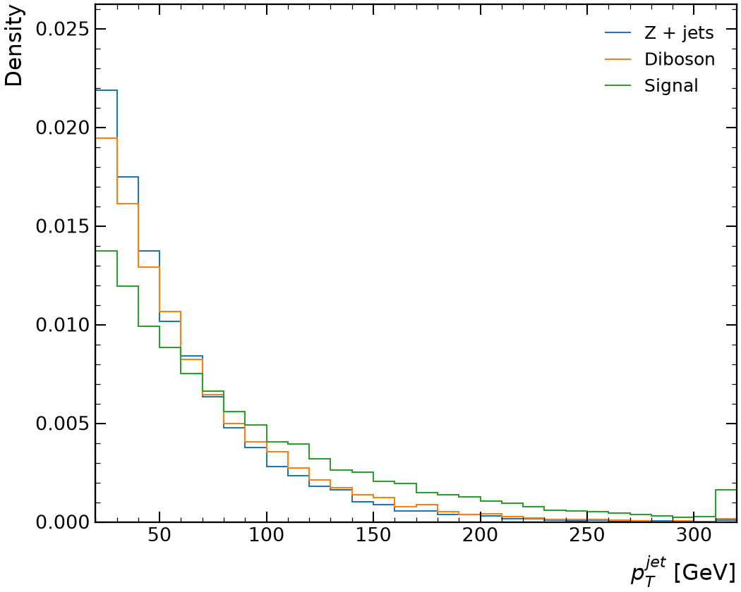
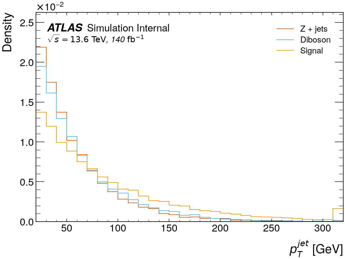
Density normalisation and summed overflow

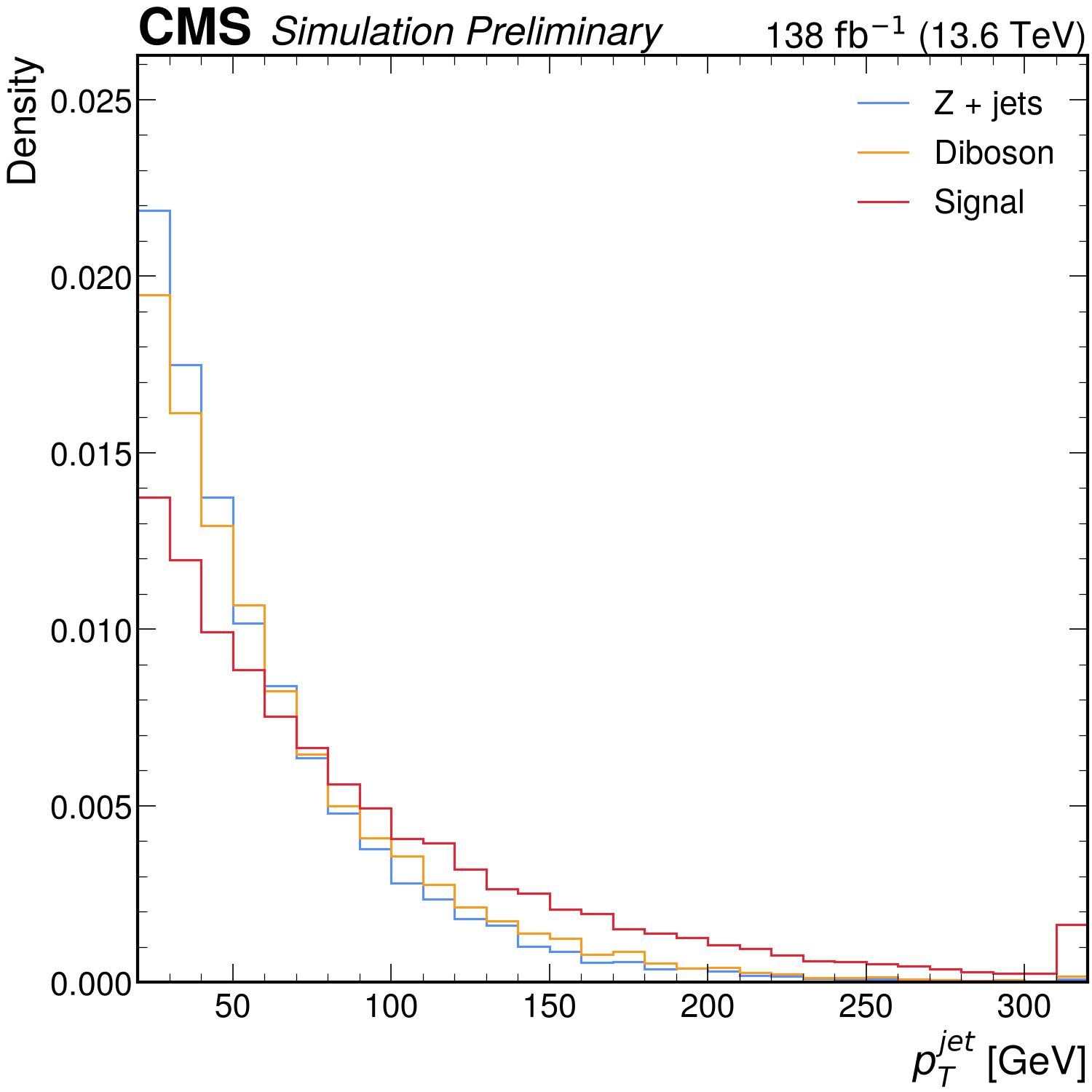
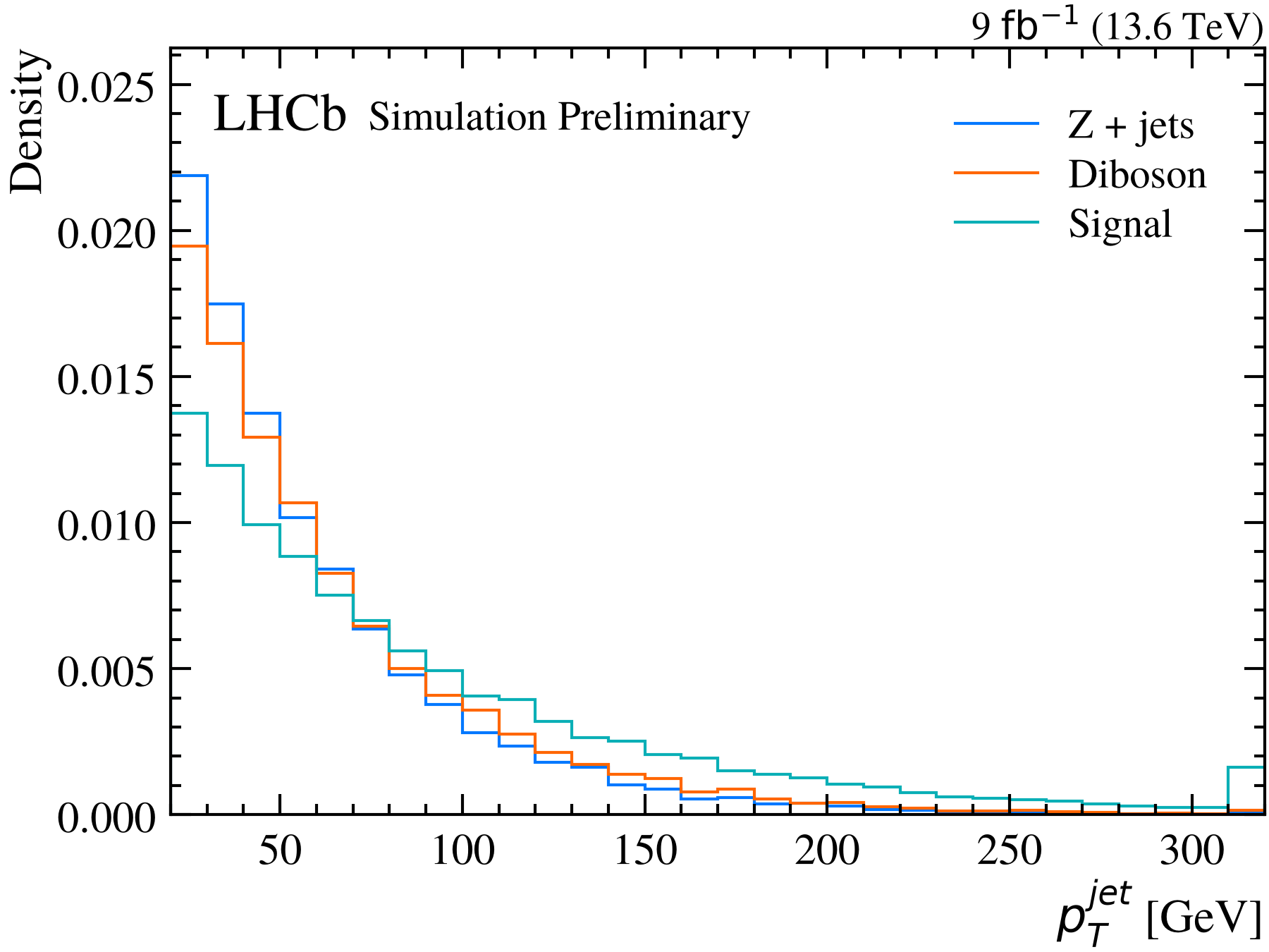
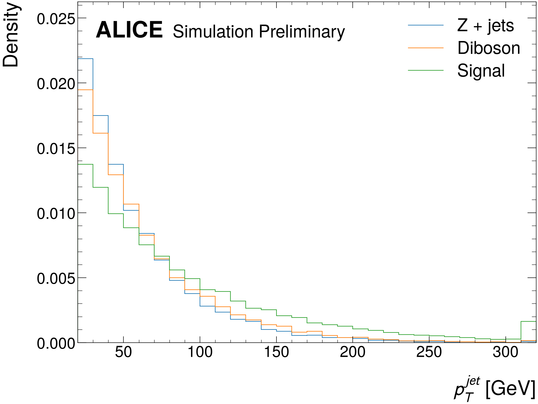
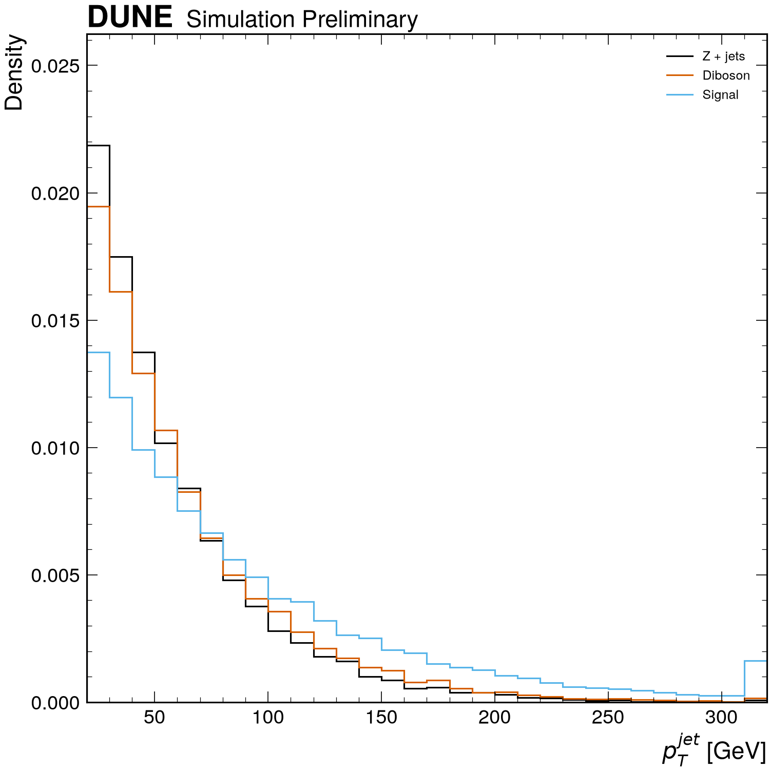
normalize="density" makes the integral one and flow="sum" adds the under- and overflow to the edge bins, which is why the last bin sticks out.

DefaultATLASCMSLHCbALICEDUNE

import rootfig as rf

style = rf.Style()

rf.plot(
    [zjets, diboson, signal],
    rf.Variable("Jet_pt", bins=(30, 20, 320), label=r"$p_T^{jet}$", unit="GeV"),
    selection="abs(Jet_eta) < 2.5",
    normalize="density",
    flow="sum",
    style=style,
)

import rootfig as rf

style = rf.Style(experiment="ATLAS", status="Internal", lumi=140, com=13.6)

rf.plot(
    [zjets, diboson, signal],
    rf.Variable("Jet_pt", bins=(30, 20, 320), label=r"$p_T^{jet}$", unit="GeV"),
    selection="abs(Jet_eta) < 2.5",
    normalize="density",
    flow="sum",
    style=style,
)

import rootfig as rf

style = rf.Style(experiment="CMS", status="Preliminary", lumi=138, com=13.6)

rf.plot(
    [zjets, diboson, signal],
    rf.Variable("Jet_pt", bins=(30, 20, 320), label=r"$p_T^{jet}$", unit="GeV"),
    selection="abs(Jet_eta) < 2.5",
    normalize="density",
    flow="sum",
    style=style,
)

import rootfig as rf

style = rf.Style(experiment="LHCb", status="Preliminary", lumi=9, com=13.6)

rf.plot(
    [zjets, diboson, signal],
    rf.Variable("Jet_pt", bins=(30, 20, 320), label=r"$p_T^{jet}$", unit="GeV"),
    selection="abs(Jet_eta) < 2.5",
    normalize="density",
    flow="sum",
    style=style,
)

import rootfig as rf

style = rf.Style(experiment="ALICE", status="Preliminary")

rf.plot(
    [zjets, diboson, signal],
    rf.Variable("Jet_pt", bins=(30, 20, 320), label=r"$p_T^{jet}$", unit="GeV"),
    selection="abs(Jet_eta) < 2.5",
    normalize="density",
    flow="sum",
    style=style,
)

import rootfig as rf

style = rf.Style(experiment="DUNE", status="Preliminary")

rf.plot(
    [zjets, diboson, signal],
    rf.Variable("Jet_pt", bins=(30, 20, 320), label=r"$p_T^{jet}$", unit="GeV"),
    selection="abs(Jet_eta) < 2.5",
    normalize="density",
    flow="sum",
    style=style,
)

Setup

The code reads the toy dataset. In a checkout of rootfig, python examples/gallery writes it to examples/out/ in a few seconds; run the code inside that directory.

It uses these samples and variables, shared by the gallery examples (see Samples, variables, cuts and styles):

signal = rf.Sample("signal.root", tree="events", label="Signal", weight="weight", scale=0.03)
zjets = rf.Sample("background.root", tree="events", label="Z + jets", weight="weight")
diboson = rf.Sample("diboson.root", tree="events", label="Diboson", weight="weight", scale=0.15)
data = rf.Sample("data.root", tree="events", label="Data", is_data=True)
mc = [zjets, diboson, signal]  # stacked bottom to top

pt = rf.Variable("Muon_pt", bins=(30, 0, 300), label=r"$p_T^{\mu}$", unit="GeV")
mll = rf.Variable("m_ll", bins=(70, 50, 260), label=r"$m_{\ell\ell}$", unit="GeV")
met = rf.Variable("MET", bins=(40, 0, 400), label=r"$E_T^{miss}$", unit="GeV")