Automatic ranges: robust by default, or the full extent
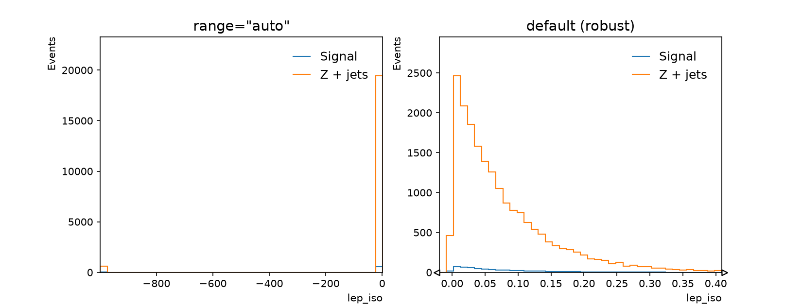
Sentinels such as -999 wreck an automatic range, so an integer bins without an
explicit range infers one robustly: far outliers are ignored when choosing the axis, and
the thin end of a tail is cut as long as few entries leave the view (nothing is removed
from the data, it ends up in the flow bins, where the arrows point at it).
range="auto" asks for the full finite minimum and maximum instead. Passing ax=
draws into your own axes, so two rootfig plots share one figure.
import matplotlib.pyplot as plt
import rootfig as rf

_, (left, right) = plt.subplots(1, 2, figsize=(11, 4.2))
rf.plot([signal, zjets], "lep_iso", bins=40, range="auto", ax=left, title='range="auto"')
rf.plot([signal, zjets], "lep_iso", bins=40, ax=right, title="default (robust)")
Setup
The code reads the toy dataset. In a checkout of rootfig, python examples/gallery writes it to examples/out/ in a few seconds; run the code inside that directory.
It uses these samples and variables, shared by the gallery examples (see Samples, variables, cuts and styles):
signal = rf.Sample("signal.root", tree="events", label="Signal", weight="weight", scale=0.03)
zjets = rf.Sample("background.root", tree="events", label="Z + jets", weight="weight")
diboson = rf.Sample("diboson.root", tree="events", label="Diboson", weight="weight", scale=0.15)
data = rf.Sample("data.root", tree="events", label="Data", is_data=True)
mc = [zjets, diboson, signal]  # stacked bottom to top

pt = rf.Variable("Muon_pt", bins=(30, 0, 300), label=r"$p_T^{\mu}$", unit="GeV")
mll = rf.Variable("m_ll", bins=(70, 50, 260), label=r"$m_{\ell\ell}$", unit="GeV")
met = rf.Variable("MET", bins=(40, 0, 400), label=r"$E_T^{miss}$", unit="GeV")