Efficiency versus a variable with binomial intervals

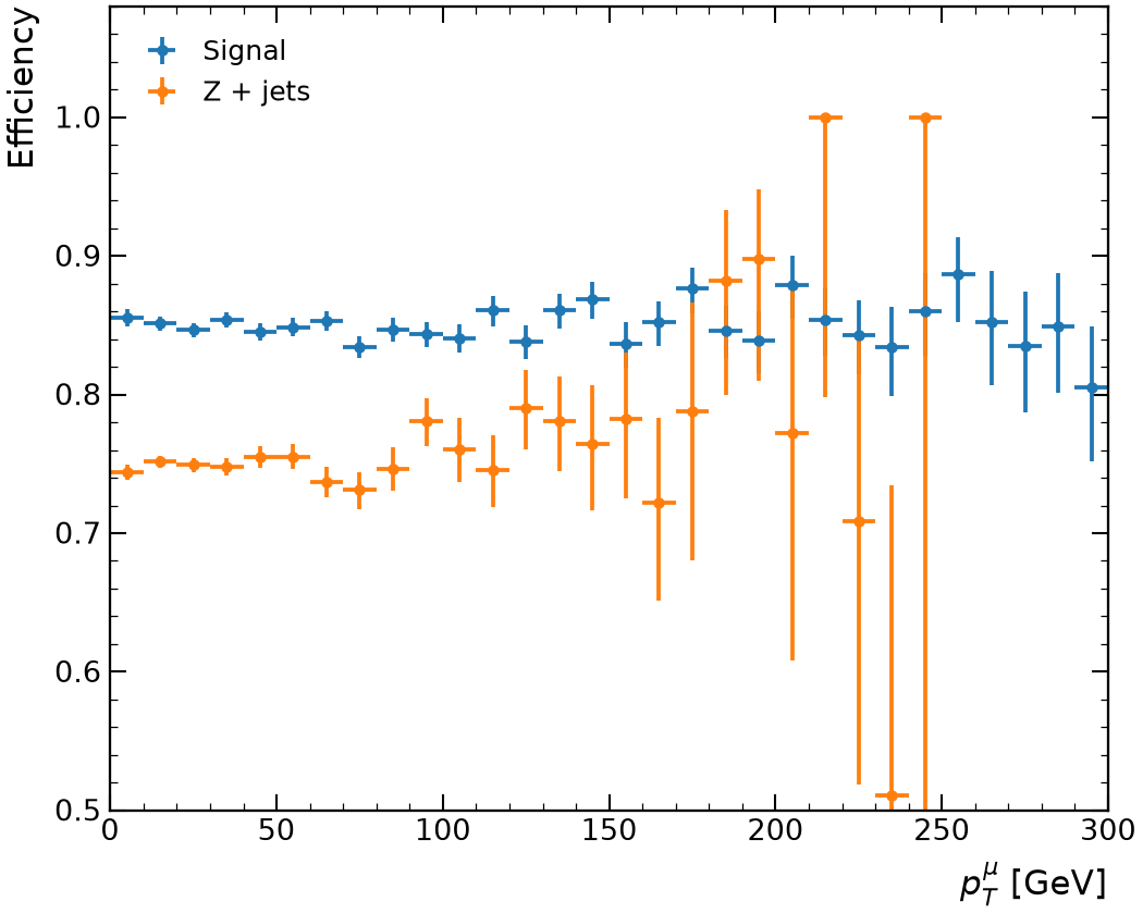
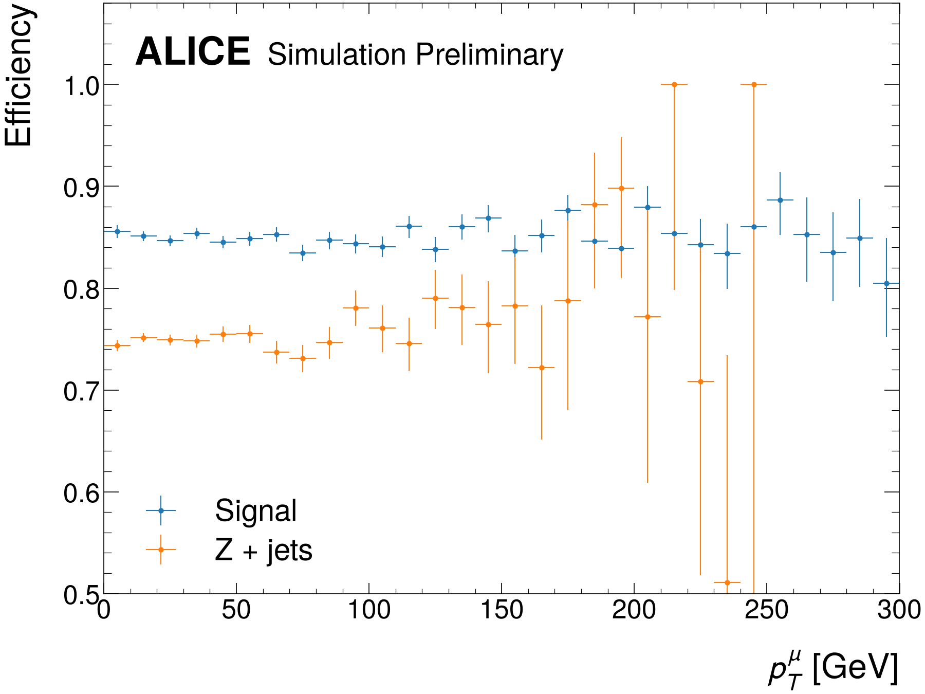
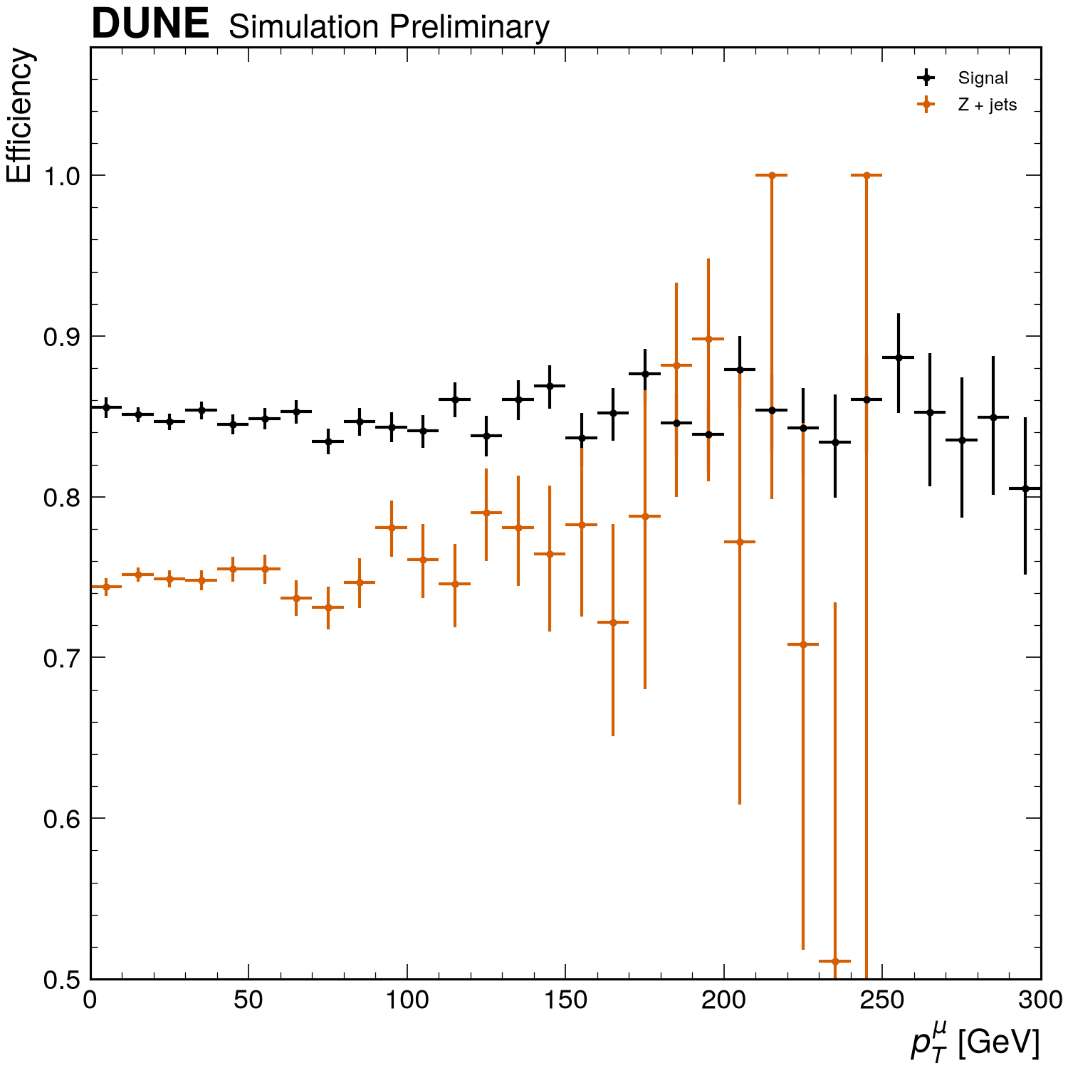
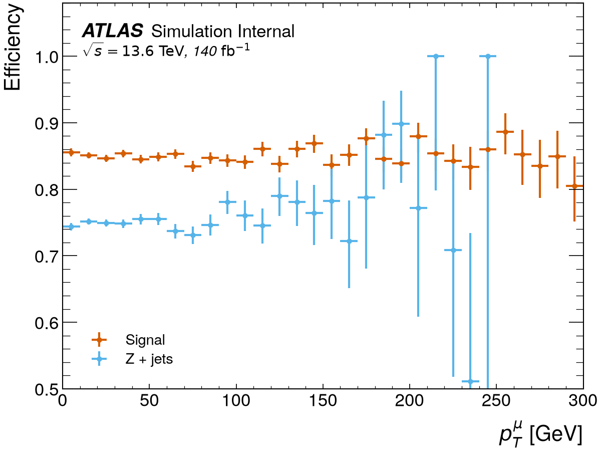
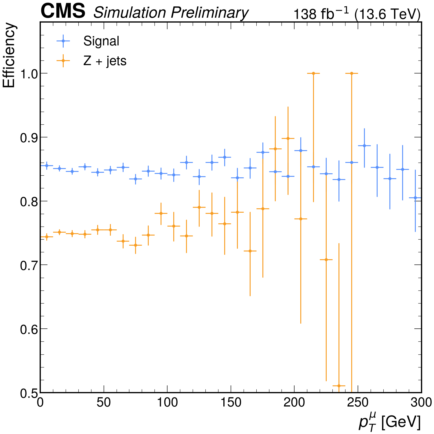
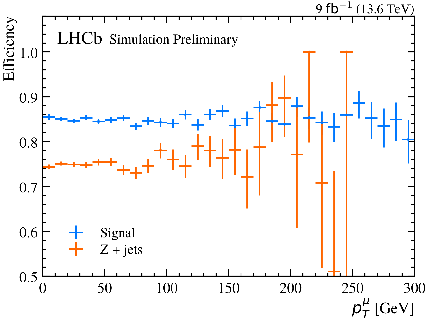
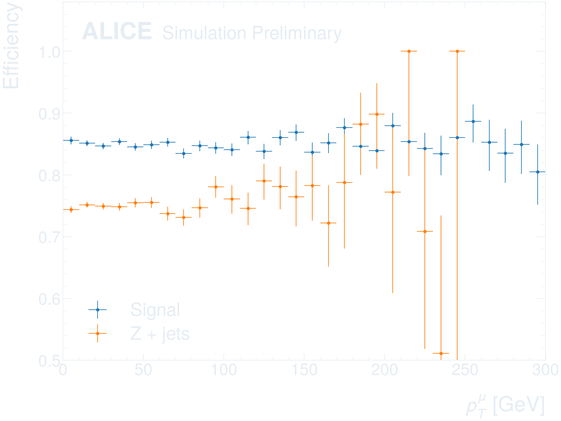
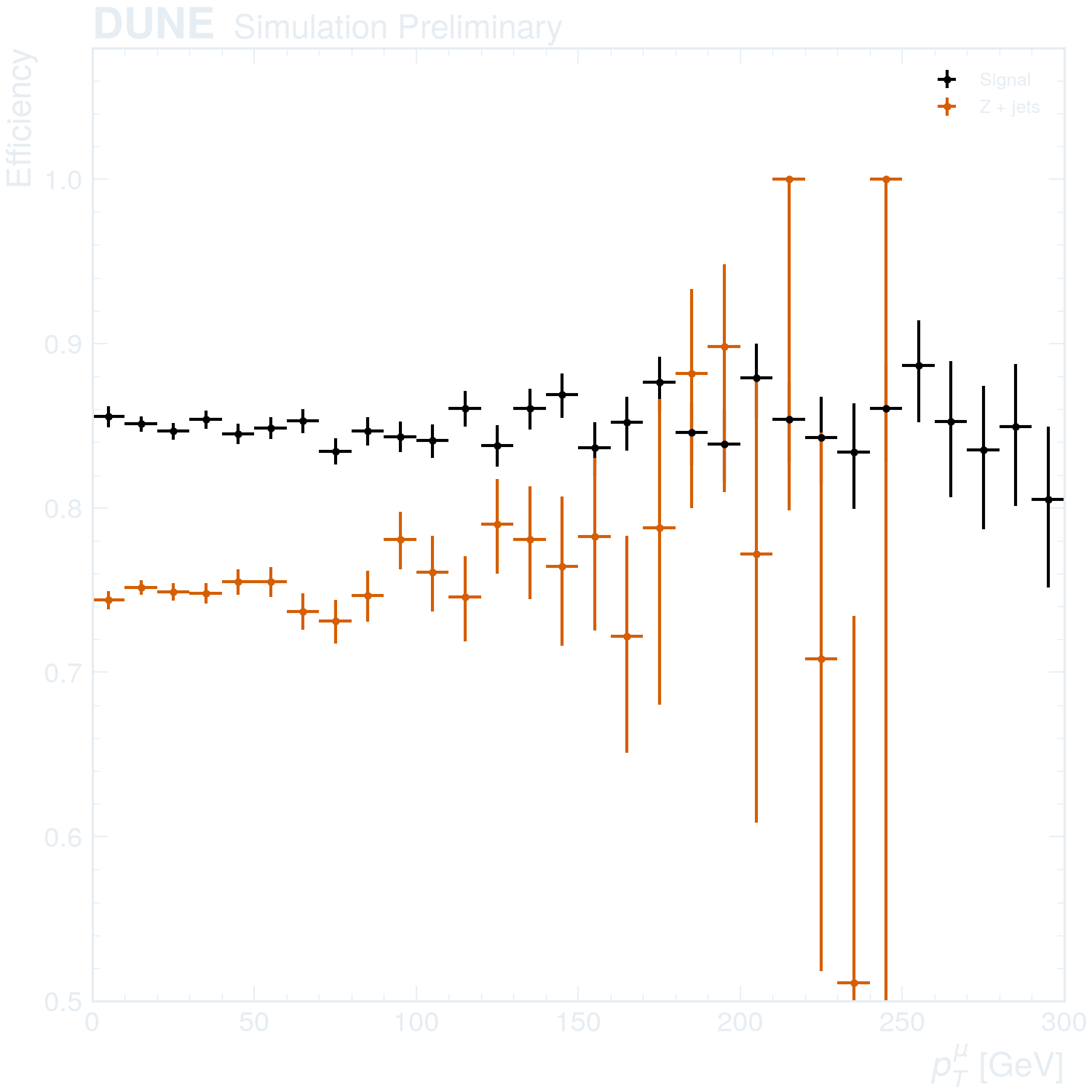
rf.efficiency fills the entries passing selection (all here) and those also passing passed with one binning, and draws their ratio with Wilson score intervals. The muon identification efficiency versus transverse momentum, for two samples.

DefaultATLASCMSLHCbALICEDUNE

import rootfig as rf

style = rf.Style()

rf.efficiency([signal, zjets], pt, passed="Muon_isTight", ylim=(0.5, None), style=style)

import rootfig as rf

style = rf.Style(experiment="ATLAS", status="Internal", lumi=140, com=13.6)

rf.efficiency([signal, zjets], pt, passed="Muon_isTight", ylim=(0.5, None), style=style)

import rootfig as rf

style = rf.Style(experiment="CMS", status="Preliminary", lumi=138, com=13.6)

rf.efficiency([signal, zjets], pt, passed="Muon_isTight", ylim=(0.5, None), style=style)

import rootfig as rf

style = rf.Style(experiment="LHCb", status="Preliminary", lumi=9, com=13.6)

rf.efficiency([signal, zjets], pt, passed="Muon_isTight", ylim=(0.5, None), style=style)

import rootfig as rf

style = rf.Style(experiment="ALICE", status="Preliminary")

rf.efficiency([signal, zjets], pt, passed="Muon_isTight", ylim=(0.5, None), style=style)

import rootfig as rf

style = rf.Style(experiment="DUNE", status="Preliminary")

rf.efficiency([signal, zjets], pt, passed="Muon_isTight", ylim=(0.5, None), style=style)

Setup

The code reads the toy dataset. In a checkout of rootfig, python examples/gallery writes it to examples/out/ in a few seconds; run the code inside that directory.

It uses these samples and variables, shared by the gallery examples (see Samples, variables, cuts and styles):

signal = rf.Sample("signal.root", tree="events", label="Signal", weight="weight", scale=0.03)
zjets = rf.Sample("background.root", tree="events", label="Z + jets", weight="weight")
diboson = rf.Sample("diboson.root", tree="events", label="Diboson", weight="weight", scale=0.15)
data = rf.Sample("data.root", tree="events", label="Data", is_data=True)
mc = [zjets, diboson, signal]  # stacked bottom to top

pt = rf.Variable("Muon_pt", bins=(30, 0, 300), label=r"$p_T^{\mu}$", unit="GeV")
mll = rf.Variable("m_ll", bins=(70, 50, 260), label=r"$m_{\ell\ell}$", unit="GeV")
met = rf.Variable("MET", bins=(40, 0, 400), label=r"$E_T^{miss}$", unit="GeV")