The one-liner
A file, a branch, a selection and a binning. rootfig reads only the branches it
needs, applies the cut to each muon and draws the result with sensible defaults.
xlabel and unit dress the axes (a Variable does the same, reusably), and
style sets the look: a Style naming an experiment brings its style sheet and
label.
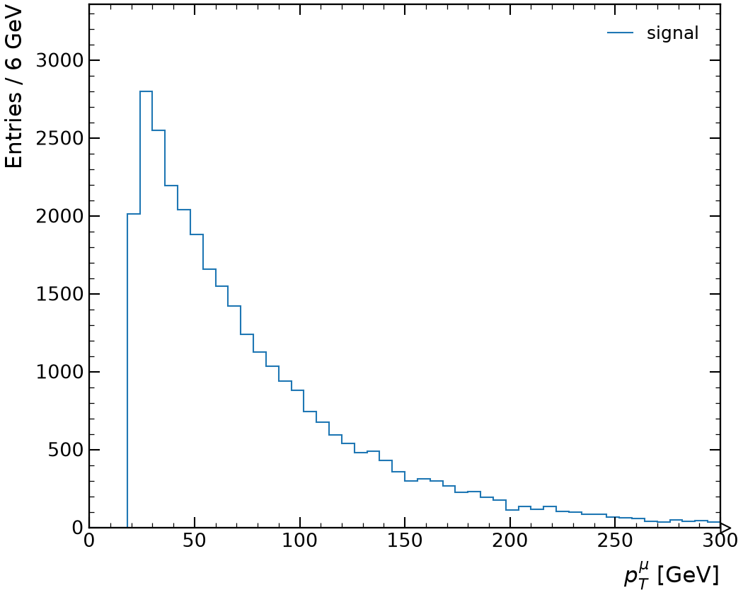
import rootfig as rf

style = rf.Style()

rf.plot(
    "signal.root",
    "Muon_pt",
    tree="events",
    selection="Muon_pt > 20",
    bins=(50, 0, 300),
    xlabel=r"$p_T^{\mu}$",
    unit="GeV",
    style=style,
)
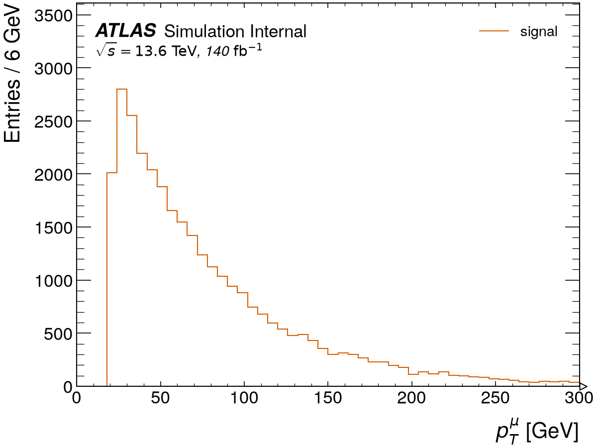
import rootfig as rf

style = rf.Style(experiment="ATLAS", status="Internal", lumi=140, com=13.6)

rf.plot(
    "signal.root",
    "Muon_pt",
    tree="events",
    selection="Muon_pt > 20",
    bins=(50, 0, 300),
    xlabel=r"$p_T^{\mu}$",
    unit="GeV",
    style=style,
)
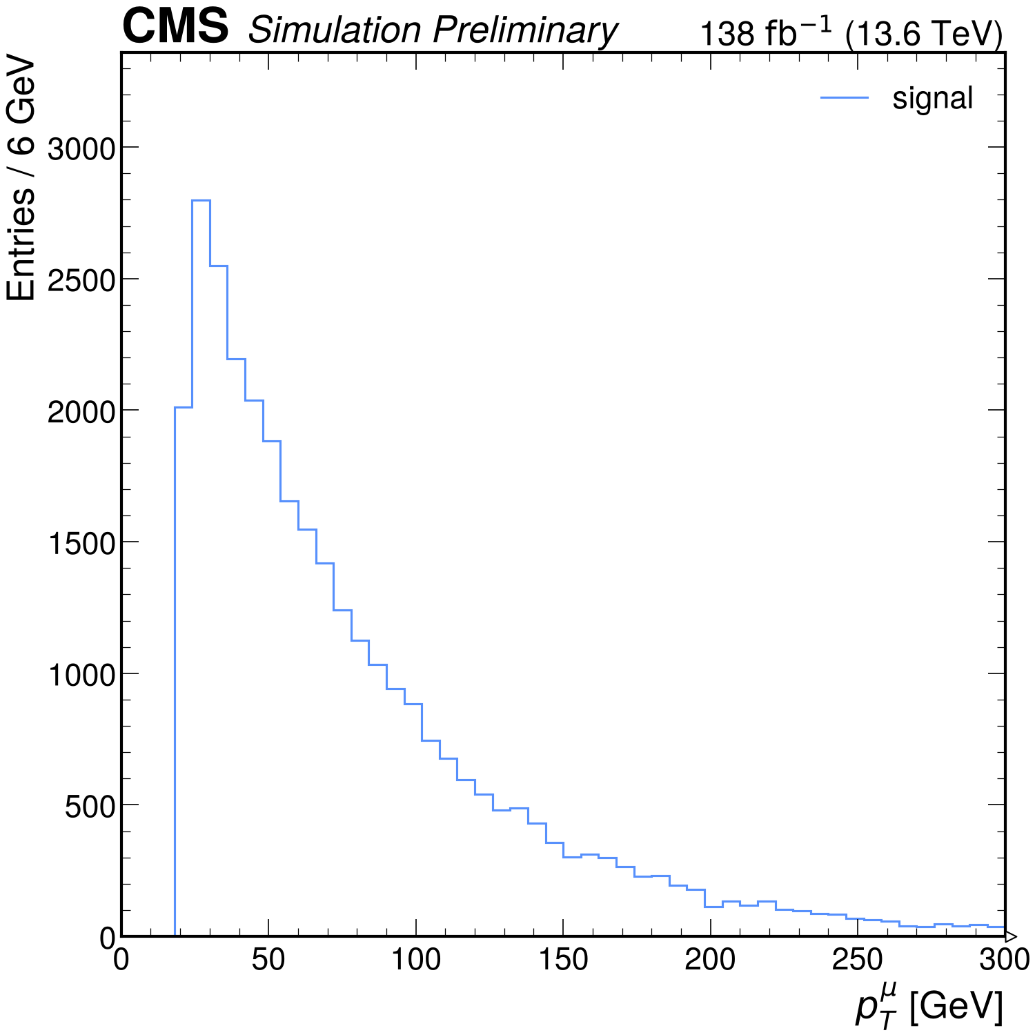
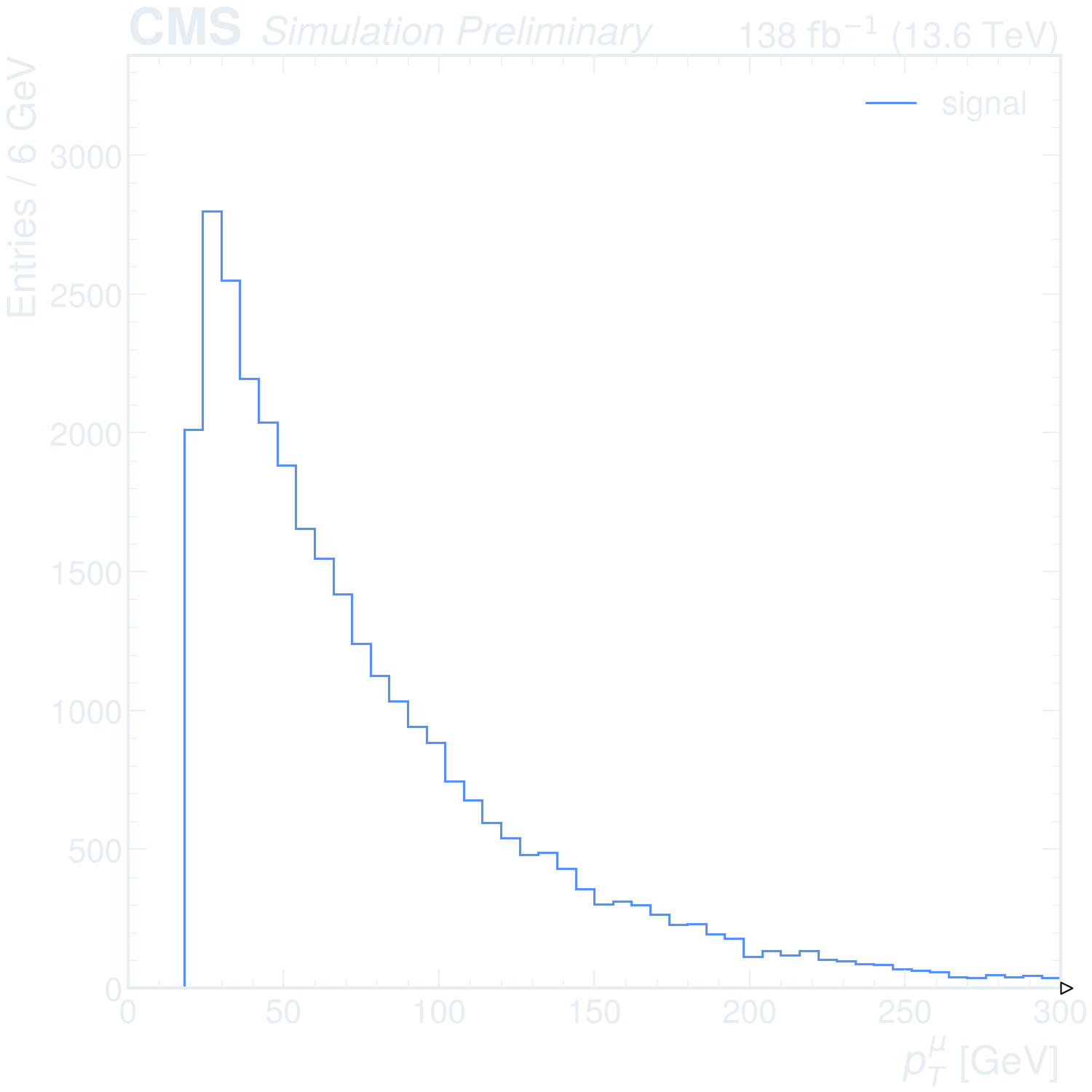
import rootfig as rf

style = rf.Style(experiment="CMS", status="Preliminary", lumi=138, com=13.6)

rf.plot(
    "signal.root",
    "Muon_pt",
    tree="events",
    selection="Muon_pt > 20",
    bins=(50, 0, 300),
    xlabel=r"$p_T^{\mu}$",
    unit="GeV",
    style=style,
)
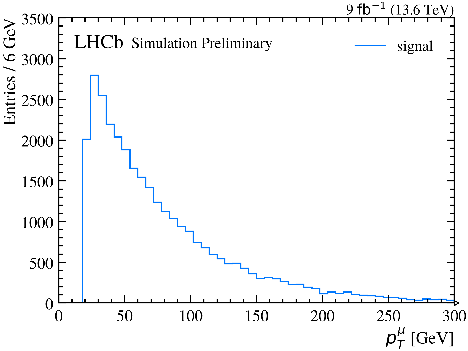
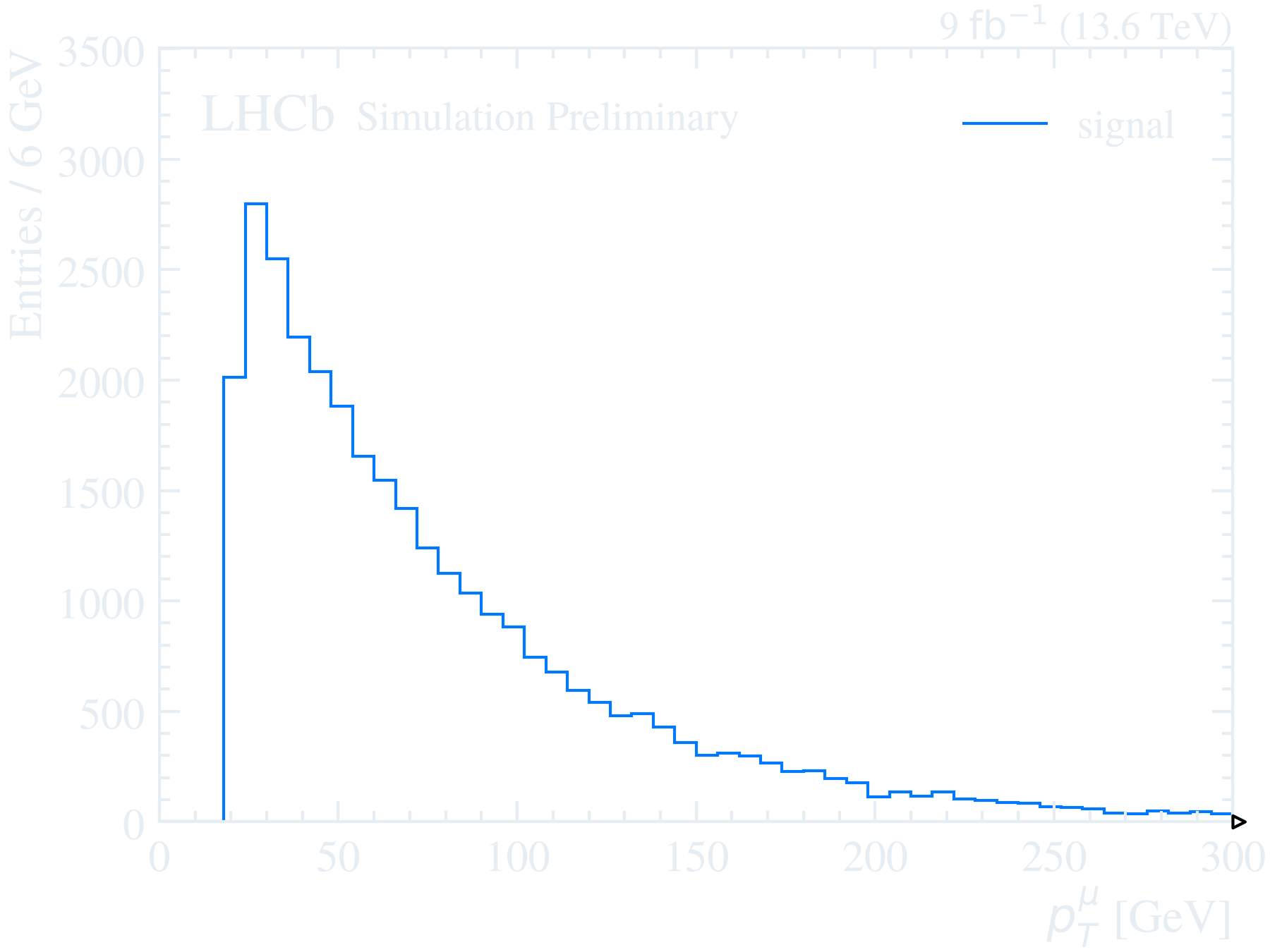
import rootfig as rf

style = rf.Style(experiment="LHCb", status="Preliminary", lumi=9, com=13.6)

rf.plot(
    "signal.root",
    "Muon_pt",
    tree="events",
    selection="Muon_pt > 20",
    bins=(50, 0, 300),
    xlabel=r"$p_T^{\mu}$",
    unit="GeV",
    style=style,
)
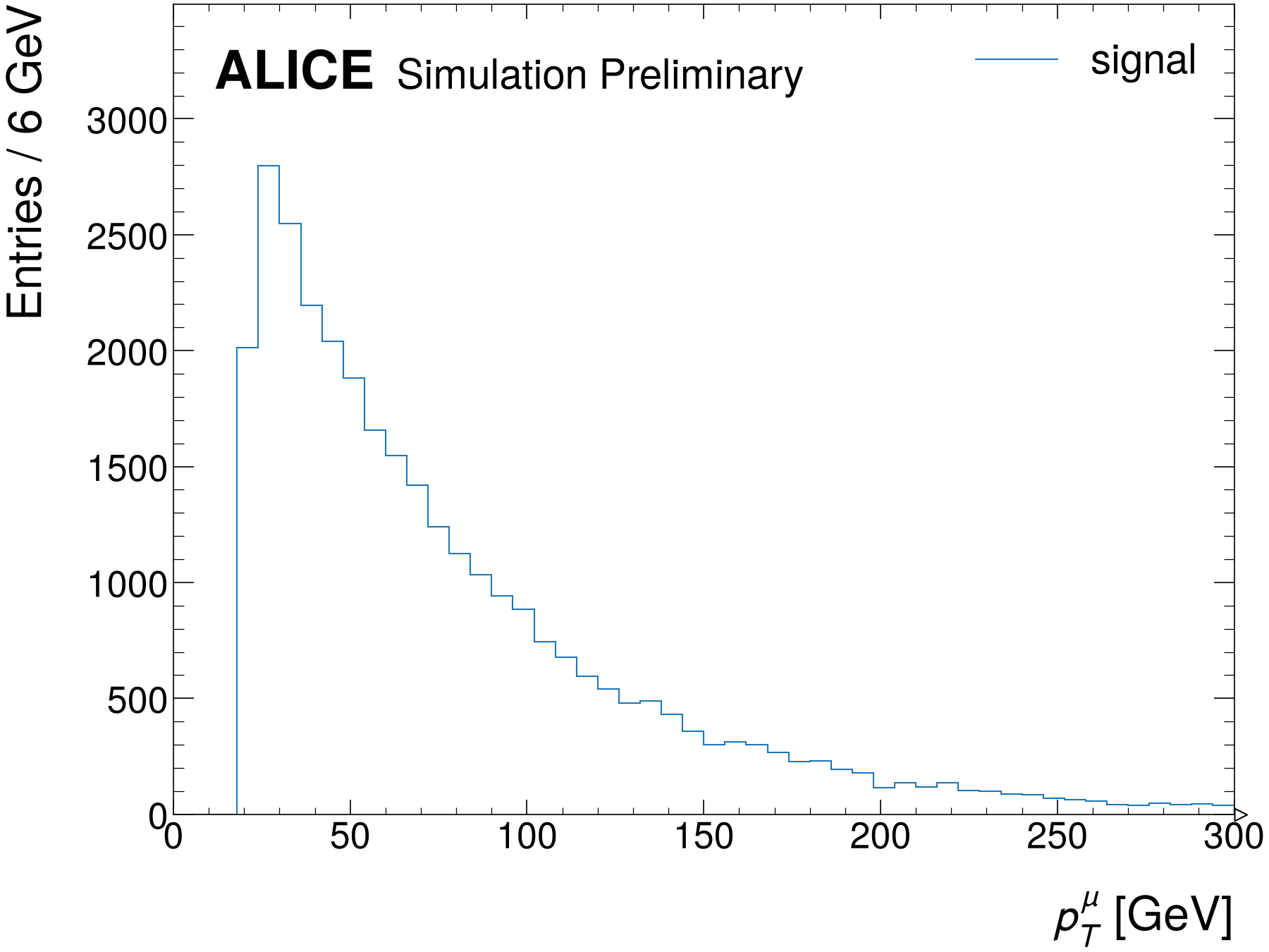
import rootfig as rf

style = rf.Style(experiment="ALICE", status="Preliminary")

rf.plot(
    "signal.root",
    "Muon_pt",
    tree="events",
    selection="Muon_pt > 20",
    bins=(50, 0, 300),
    xlabel=r"$p_T^{\mu}$",
    unit="GeV",
    style=style,
)
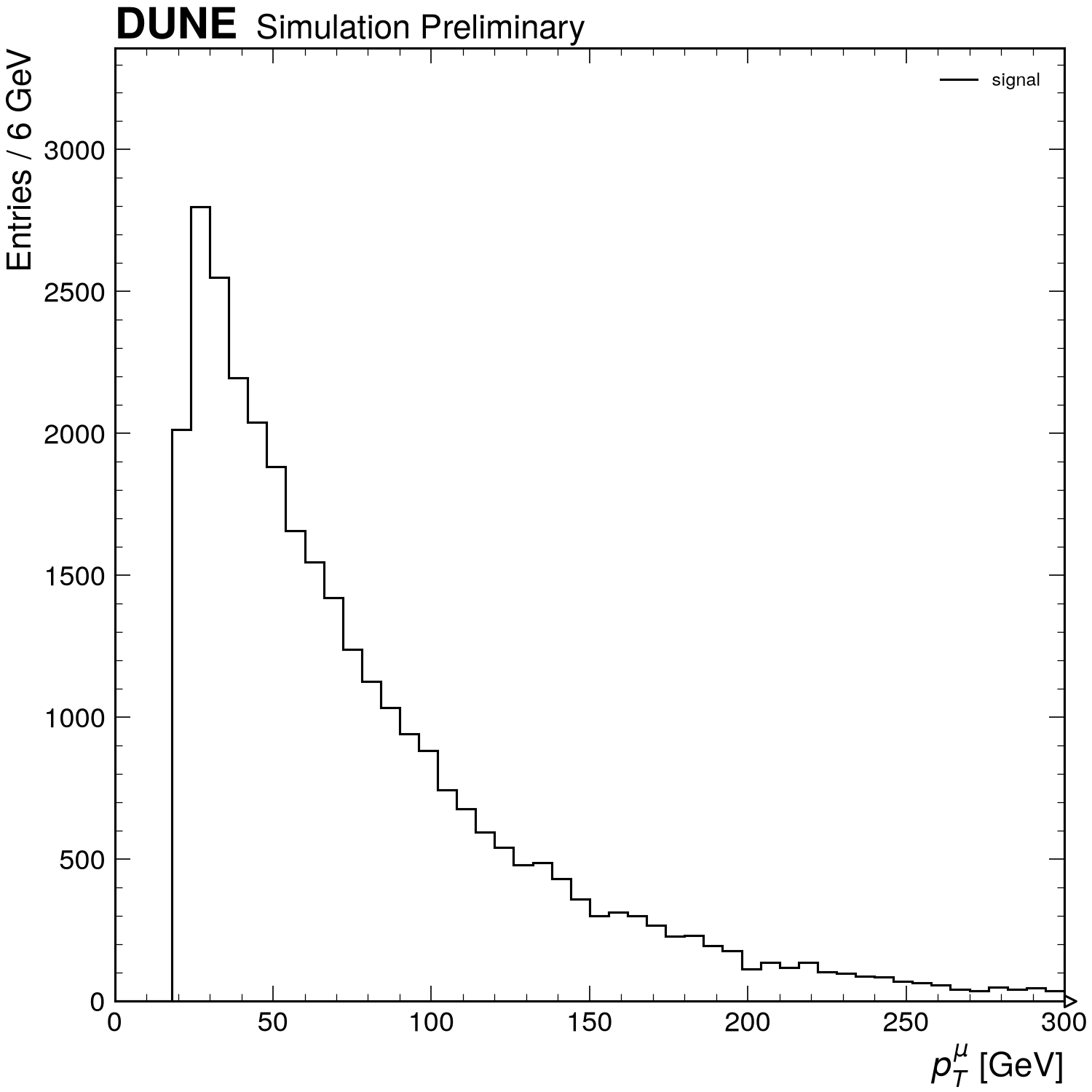
import rootfig as rf

style = rf.Style(experiment="DUNE", status="Preliminary")

rf.plot(
    "signal.root",
    "Muon_pt",
    tree="events",
    selection="Muon_pt > 20",
    bins=(50, 0, 300),
    xlabel=r"$p_T^{\mu}$",
    unit="GeV",
    style=style,
)
Setup
The code reads the toy dataset. In a checkout of rootfig, python examples/gallery writes it to examples/out/ in a few seconds; run the code inside that directory.