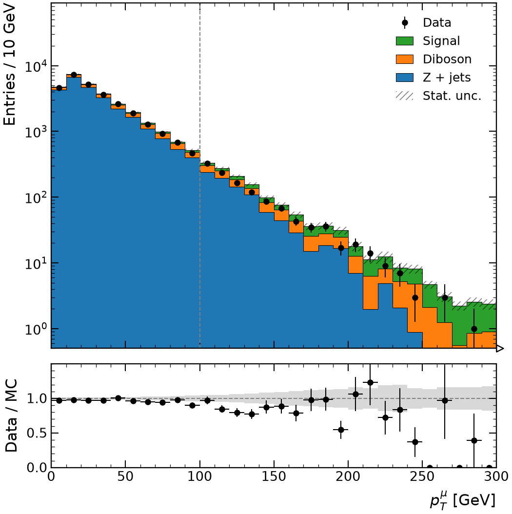
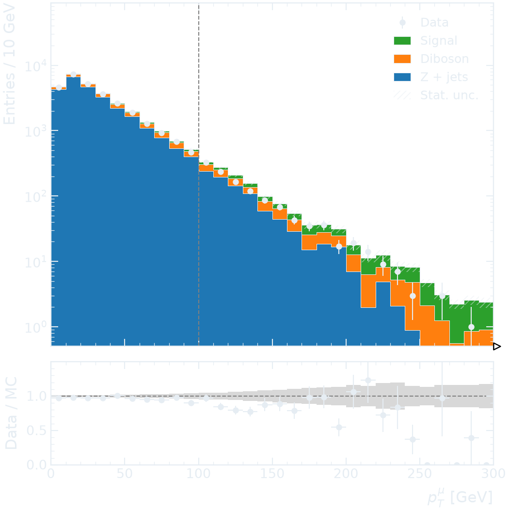
Stacked simulation with data and a ratio panel

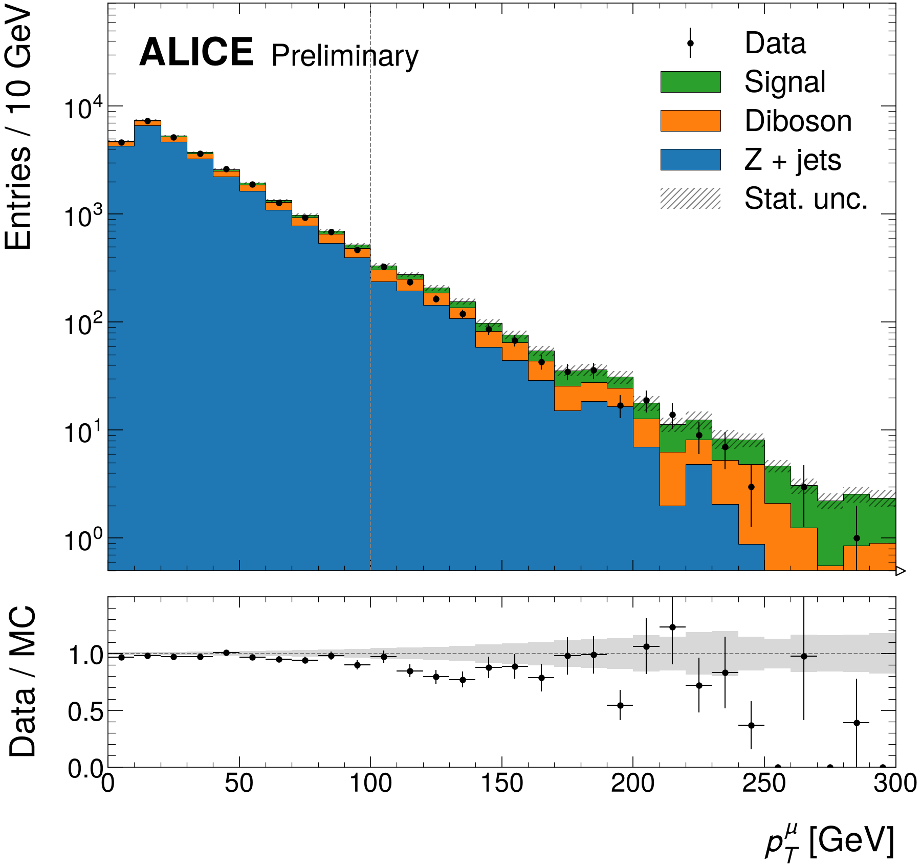
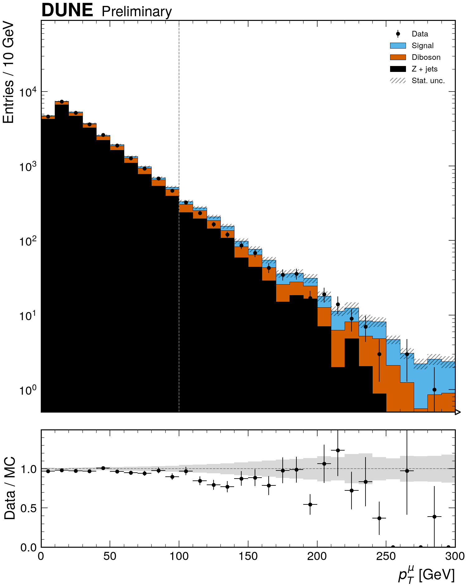
A Cut combines selection strings with & and carries a label for the plot. Simulation is stacked bottom to top in the given order with a hatched statistical-uncertainty band, data is drawn as points, and the ratio panel shows data over the total prediction. The returned Plot holds plain matplotlib objects, so any further customisation is ordinary matplotlib code.

DefaultATLASCMSLHCbALICEDUNE

import rootfig as rf

style = rf.Style()

tight = rf.Cut("Muon_isTight", label="tight") & "abs(Muon_eta) < 2.5"
p = rf.plot(
    mc, pt, observed=data, selection=tight, stack=True, ratio=True, logy=True, style=style
)
p.ax.axvline(100, color="gray", linestyle="--", linewidth=1)

import rootfig as rf

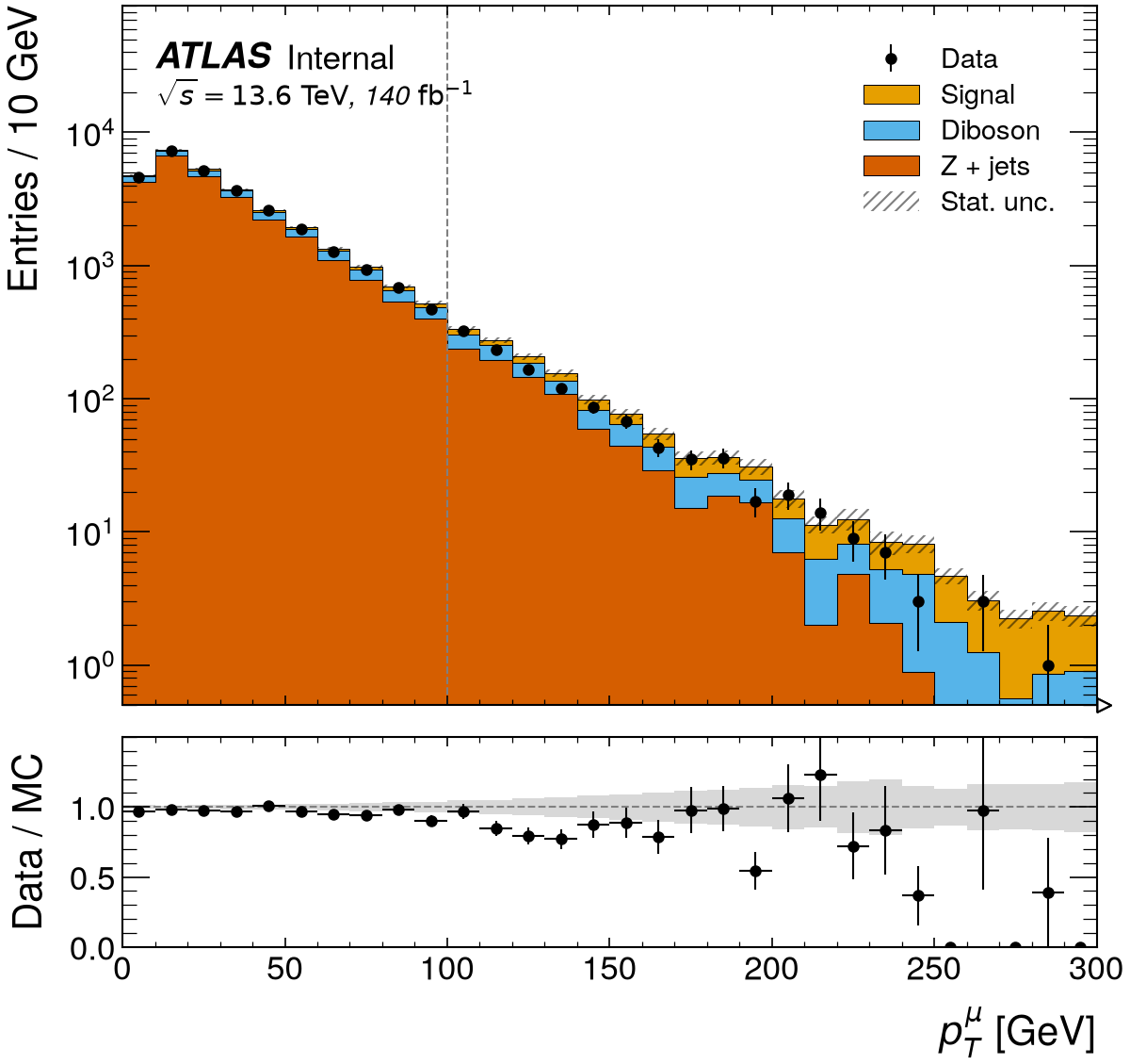
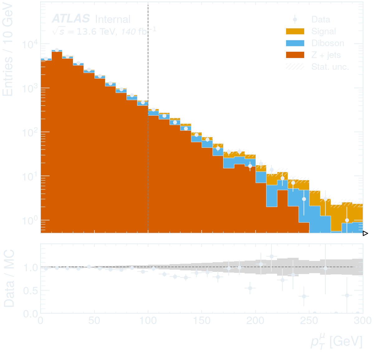
style = rf.Style(experiment="ATLAS", status="Internal", lumi=140, com=13.6)

tight = rf.Cut("Muon_isTight", label="tight") & "abs(Muon_eta) < 2.5"
p = rf.plot(
    mc, pt, observed=data, selection=tight, stack=True, ratio=True, logy=True, style=style
)
p.ax.axvline(100, color="gray", linestyle="--", linewidth=1)

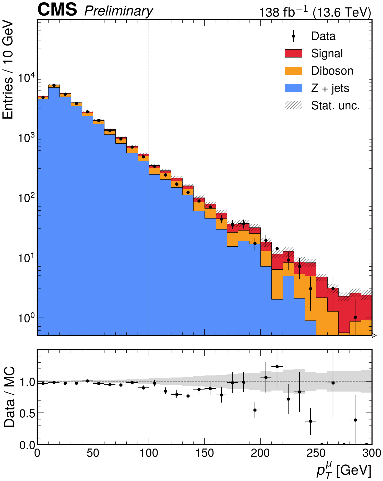
import rootfig as rf

style = rf.Style(experiment="CMS", status="Preliminary", lumi=138, com=13.6)

tight = rf.Cut("Muon_isTight", label="tight") & "abs(Muon_eta) < 2.5"
p = rf.plot(
    mc, pt, observed=data, selection=tight, stack=True, ratio=True, logy=True, style=style
)
p.ax.axvline(100, color="gray", linestyle="--", linewidth=1)

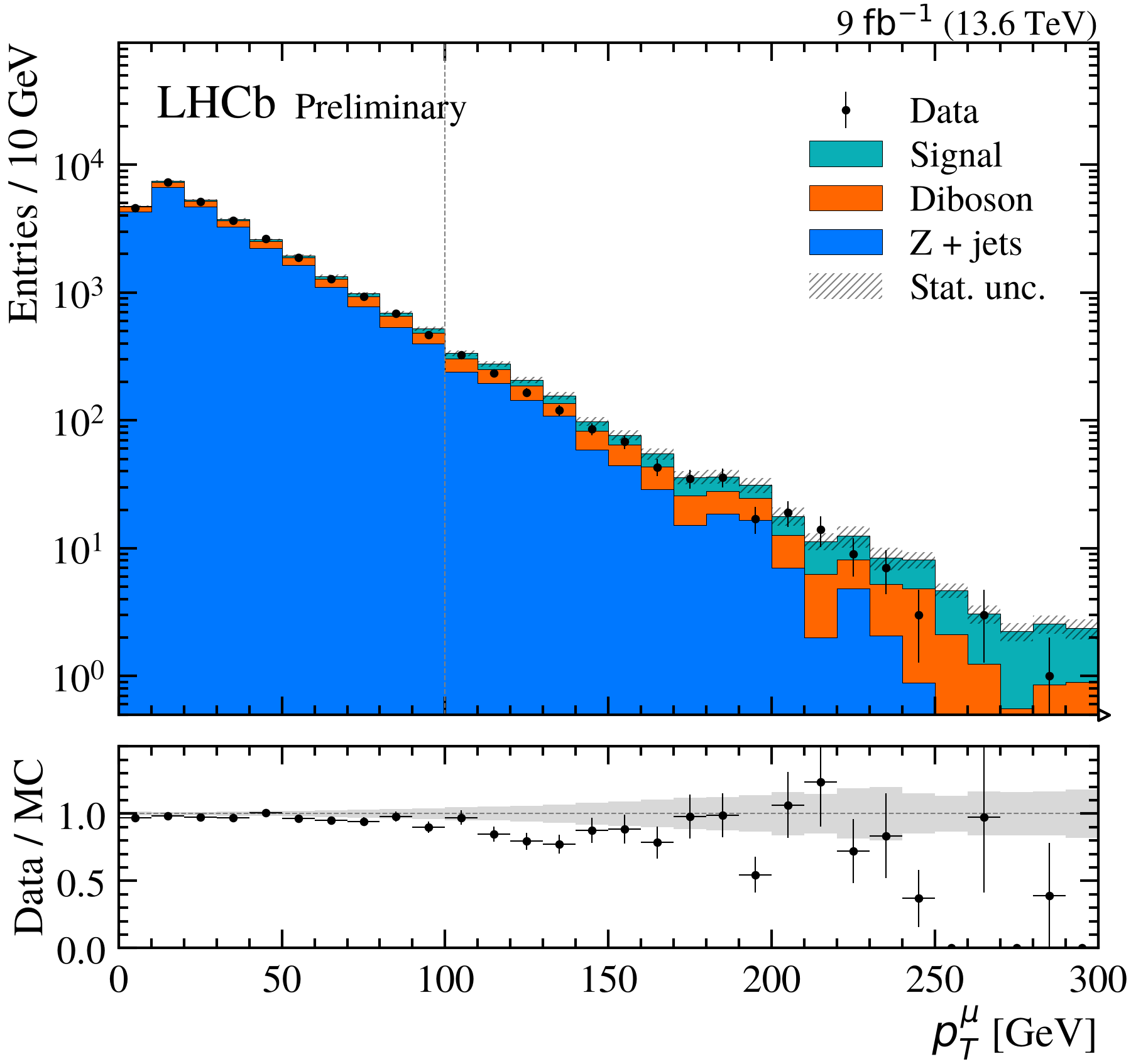
import rootfig as rf

style = rf.Style(experiment="LHCb", status="Preliminary", lumi=9, com=13.6)

tight = rf.Cut("Muon_isTight", label="tight") & "abs(Muon_eta) < 2.5"
p = rf.plot(
    mc, pt, observed=data, selection=tight, stack=True, ratio=True, logy=True, style=style
)
p.ax.axvline(100, color="gray", linestyle="--", linewidth=1)

import rootfig as rf

style = rf.Style(experiment="ALICE", status="Preliminary")

tight = rf.Cut("Muon_isTight", label="tight") & "abs(Muon_eta) < 2.5"
p = rf.plot(
    mc, pt, observed=data, selection=tight, stack=True, ratio=True, logy=True, style=style
)
p.ax.axvline(100, color="gray", linestyle="--", linewidth=1)

import rootfig as rf

style = rf.Style(experiment="DUNE", status="Preliminary")

tight = rf.Cut("Muon_isTight", label="tight") & "abs(Muon_eta) < 2.5"
p = rf.plot(
    mc, pt, observed=data, selection=tight, stack=True, ratio=True, logy=True, style=style
)
p.ax.axvline(100, color="gray", linestyle="--", linewidth=1)

Setup

The code reads the toy dataset. In a checkout of rootfig, python examples/gallery writes it to examples/out/ in a few seconds; run the code inside that directory.

It uses these samples and variables, shared by the gallery examples (see Samples, variables, cuts and styles):

signal = rf.Sample("signal.root", tree="events", label="Signal", weight="weight", scale=0.03)
zjets = rf.Sample("background.root", tree="events", label="Z + jets", weight="weight")
diboson = rf.Sample("diboson.root", tree="events", label="Diboson", weight="weight", scale=0.15)
data = rf.Sample("data.root", tree="events", label="Data", is_data=True)
mc = [zjets, diboson, signal]  # stacked bottom to top

pt = rf.Variable("Muon_pt", bins=(30, 0, 300), label=r"$p_T^{\mu}$", unit="GeV")
mll = rf.Variable("m_ll", bins=(70, 50, 260), label=r"$m_{\ell\ell}$", unit="GeV")
met = rf.Variable("MET", bins=(40, 0, 400), label=r"$E_T^{miss}$", unit="GeV")