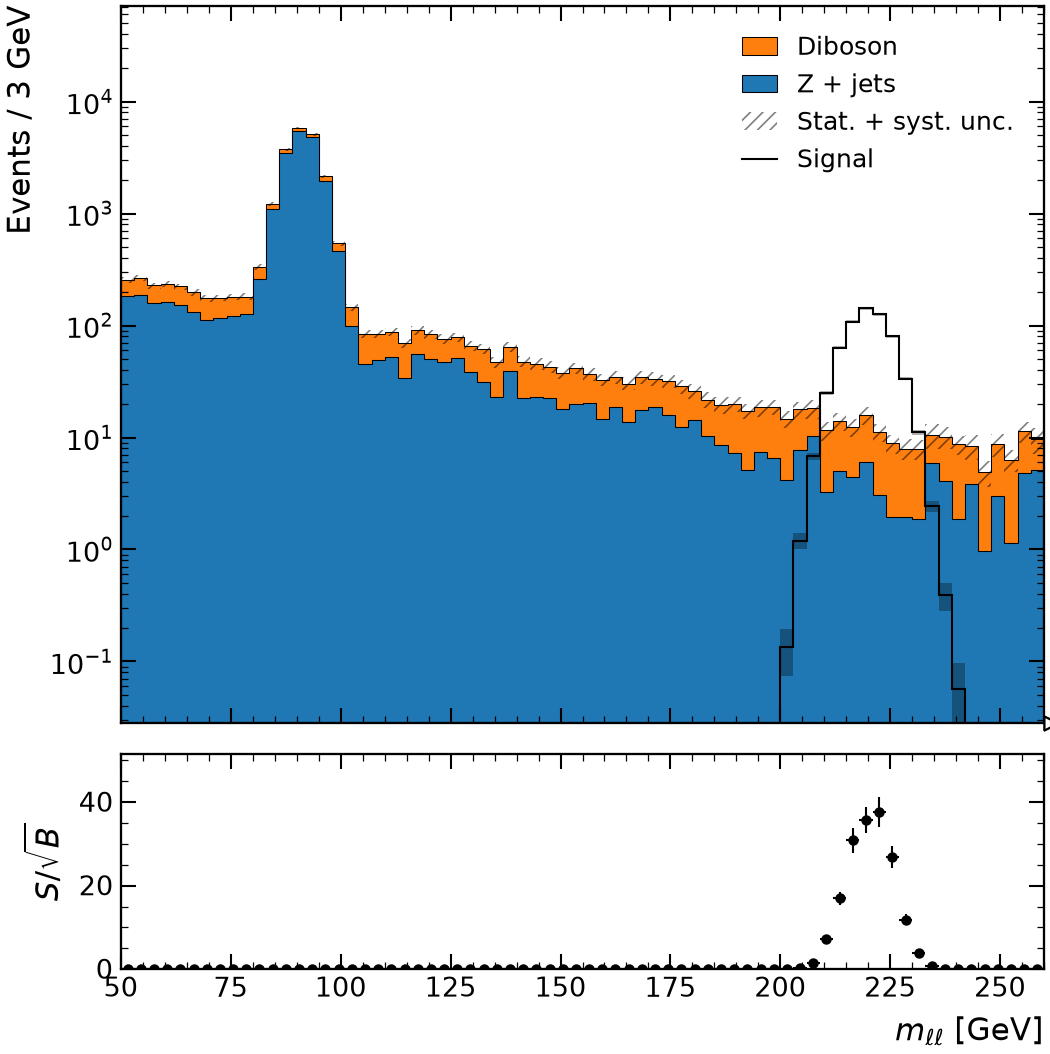
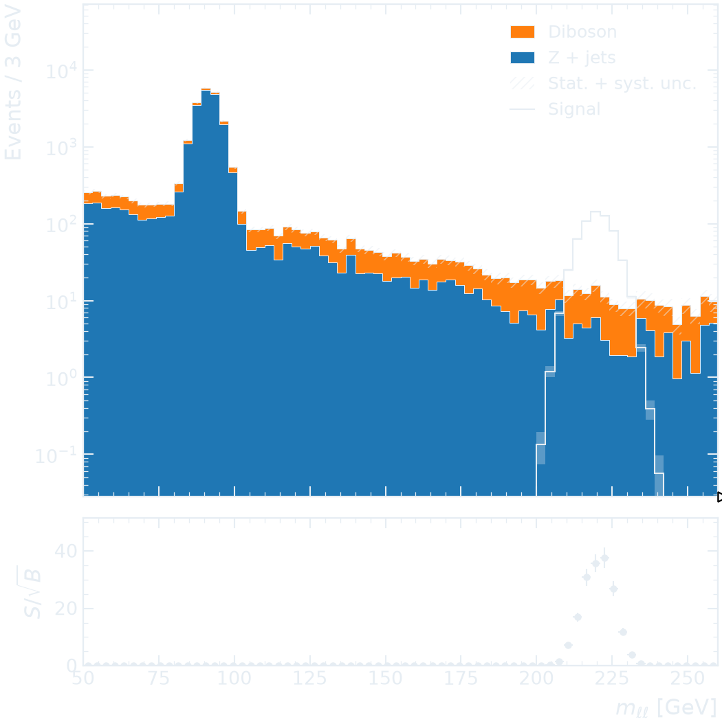
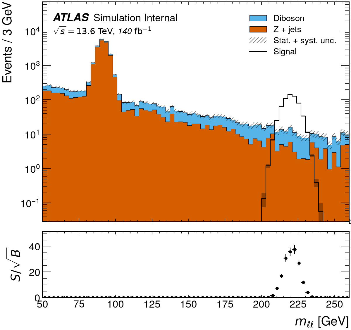
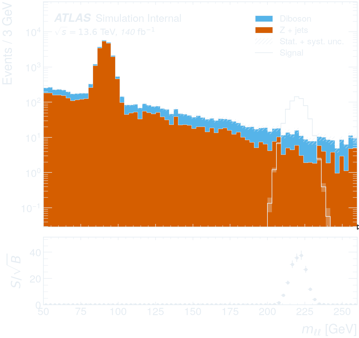
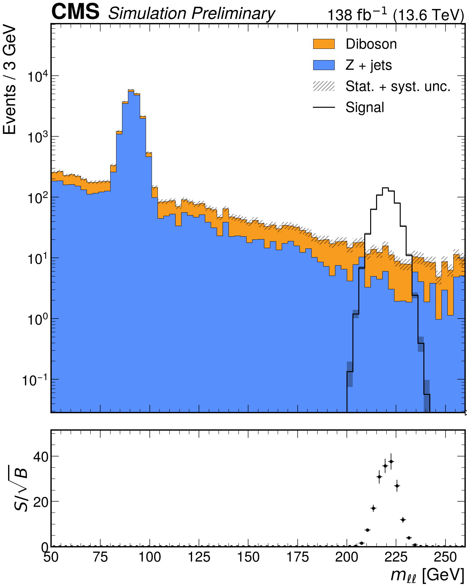
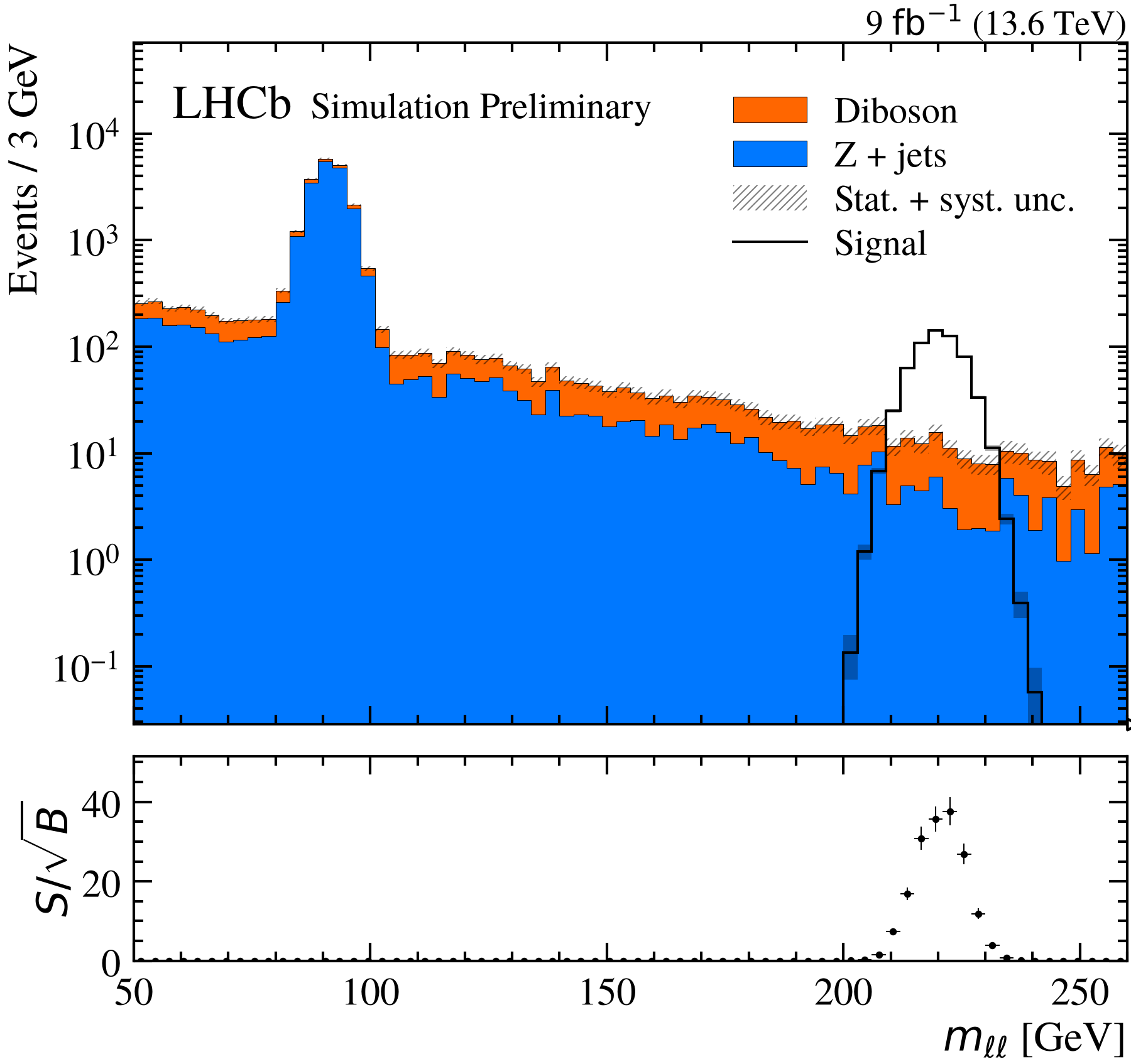
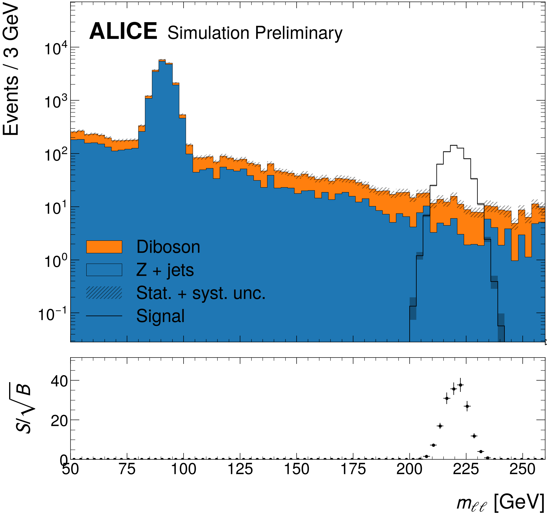
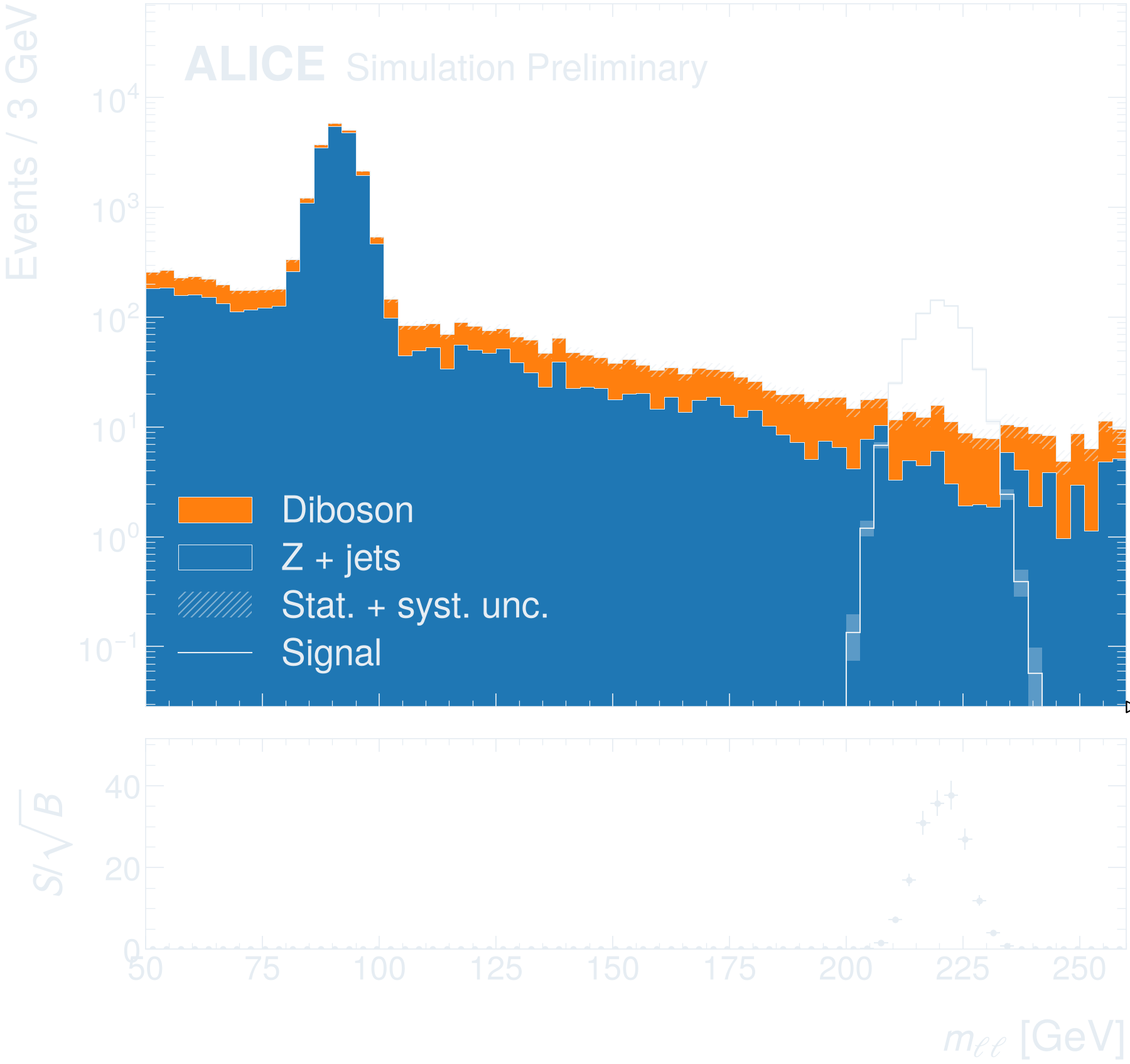
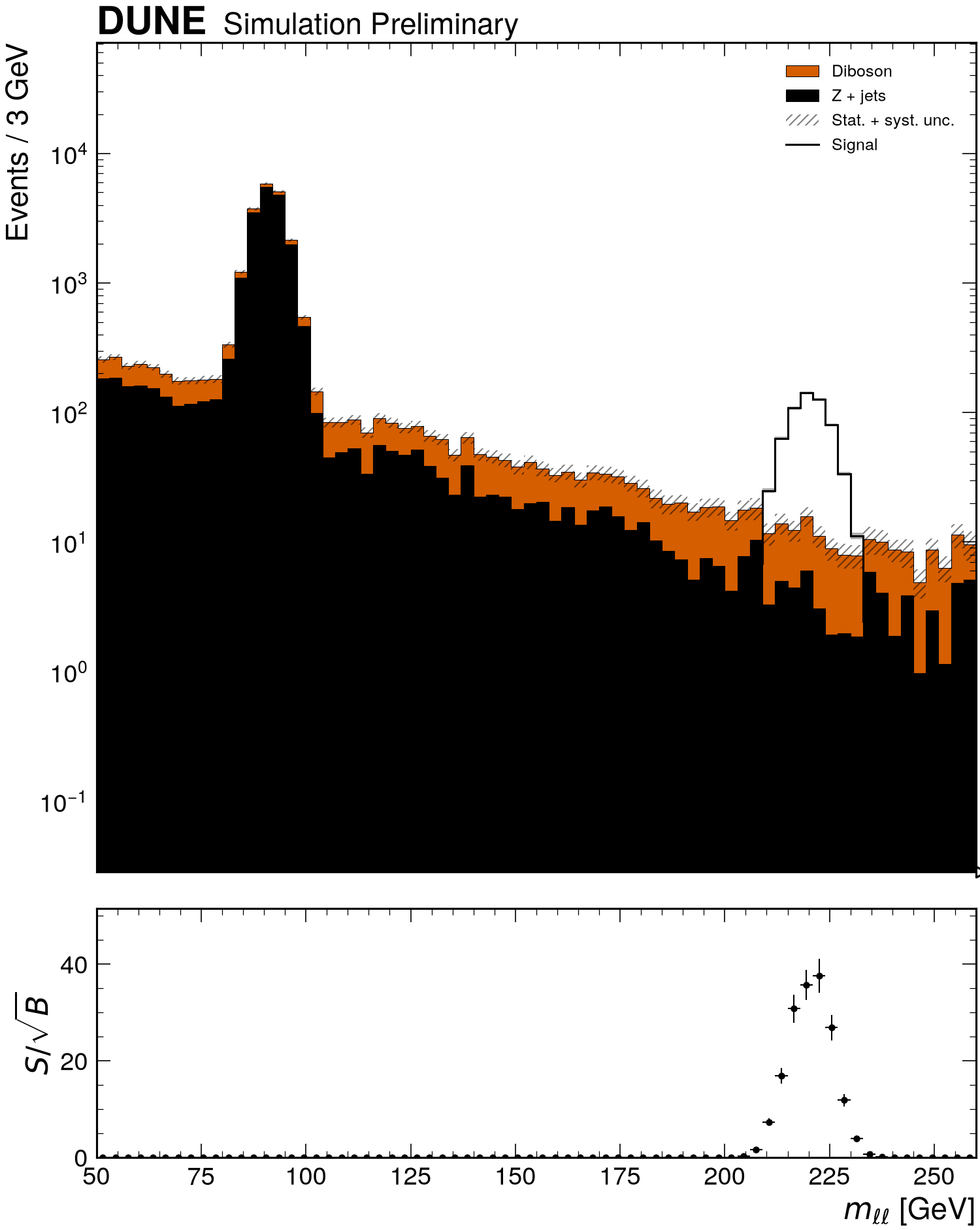
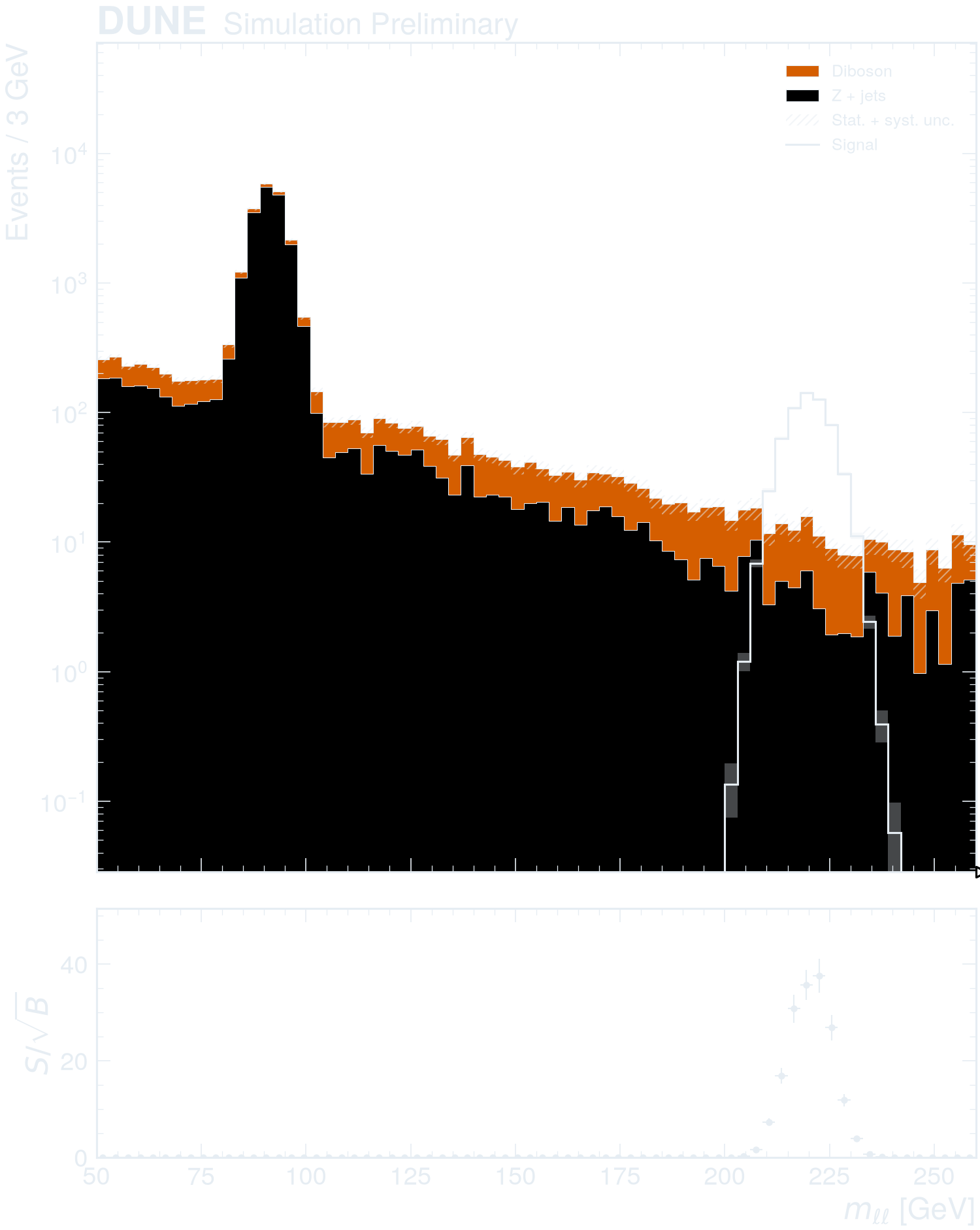
Stacked backgrounds with a signal overlaid

stack= selects the backgrounds by their legend labels. The signal is drawn as an outline over the stack in the text colour, like data points, so it stands out from the filled backgrounds on light and dark pages; panel="s/sqrt(b)" compares it with the background total, in the same colour. The hatched band belongs to the backgrounds; the signal's uncertainty is a light band in its own colour.

DefaultATLASCMSLHCbALICEDUNE

import matplotlib.pyplot as plt
import rootfig as rf

style = rf.Style()

rf.plot(
    [zjets, diboson, signal.replace(color=plt.rcParams["text.color"])],
    mll,
    stack=["Z + jets", "Diboson"],
    panel="s/sqrt(b)",
    logy=True,
    systematics={"lumi": 0.02},
    style=style,
)

import matplotlib.pyplot as plt
import rootfig as rf

style = rf.Style(experiment="ATLAS", status="Internal", lumi=140, com=13.6)

rf.plot(
    [zjets, diboson, signal.replace(color=plt.rcParams["text.color"])],
    mll,
    stack=["Z + jets", "Diboson"],
    panel="s/sqrt(b)",
    logy=True,
    systematics={"lumi": 0.02},
    style=style,
)

import matplotlib.pyplot as plt
import rootfig as rf

style = rf.Style(experiment="CMS", status="Preliminary", lumi=138, com=13.6)

rf.plot(
    [zjets, diboson, signal.replace(color=plt.rcParams["text.color"])],
    mll,
    stack=["Z + jets", "Diboson"],
    panel="s/sqrt(b)",
    logy=True,
    systematics={"lumi": 0.02},
    style=style,
)

import matplotlib.pyplot as plt
import rootfig as rf

style = rf.Style(experiment="LHCb", status="Preliminary", lumi=9, com=13.6)

rf.plot(
    [zjets, diboson, signal.replace(color=plt.rcParams["text.color"])],
    mll,
    stack=["Z + jets", "Diboson"],
    panel="s/sqrt(b)",
    logy=True,
    systematics={"lumi": 0.02},
    style=style,
)

import matplotlib.pyplot as plt
import rootfig as rf

style = rf.Style(experiment="ALICE", status="Preliminary")

rf.plot(
    [zjets, diboson, signal.replace(color=plt.rcParams["text.color"])],
    mll,
    stack=["Z + jets", "Diboson"],
    panel="s/sqrt(b)",
    logy=True,
    systematics={"lumi": 0.02},
    style=style,
)

import matplotlib.pyplot as plt
import rootfig as rf

style = rf.Style(experiment="DUNE", status="Preliminary")

rf.plot(
    [zjets, diboson, signal.replace(color=plt.rcParams["text.color"])],
    mll,
    stack=["Z + jets", "Diboson"],
    panel="s/sqrt(b)",
    logy=True,
    systematics={"lumi": 0.02},
    style=style,
)

Setup

The code reads the toy dataset. In a checkout of rootfig, python examples/gallery writes it to examples/out/ in a few seconds; run the code inside that directory.

It uses these samples and variables, shared by the gallery examples (see Samples, variables, cuts and styles):

signal = rf.Sample("signal.root", tree="events", label="Signal", weight="weight", scale=0.03)
zjets = rf.Sample("background.root", tree="events", label="Z + jets", weight="weight")
diboson = rf.Sample("diboson.root", tree="events", label="Diboson", weight="weight", scale=0.15)
data = rf.Sample("data.root", tree="events", label="Data", is_data=True)
mc = [zjets, diboson, signal]  # stacked bottom to top

pt = rf.Variable("Muon_pt", bins=(30, 0, 300), label=r"$p_T^{\mu}$", unit="GeV")
mll = rf.Variable("m_ll", bins=(70, 50, 260), label=r"$m_{\ell\ell}$", unit="GeV")
met = rf.Variable("MET", bins=(40, 0, 400), label=r"$E_T^{miss}$", unit="GeV")